Using Sensor Technologies for More Accurate Crop Estimation

by Terry Bates, Luke Haggerty, Kevin Martin, Rhiann Jakubowski

Crop load management and crop estimation are central to control risk and maintain quality. Sensors technologies have the ability to gather relative vine size, soil, and yield data. The industry-based advisory committee has identified an opportunity to have the Lake Erie Regional Grape Program diagnose problems identified by sensor technologies in grower vineyards as the next critical step toward sensor technology commercialization. In this article we show an example of how sensor data and precision agriculture offer an opportunity to accurately estimate crop and continue to maintain the intensive management control that maximize yields and maintain vine balance. As long as bulk juice prices grow slower than inflation, the industry will depend on sustainable growth of vineyards to allow growers to farm full-time through multiple generations.

Sensor technology and GIS mapping projects continue to capitalize on recent research of sensors and software that gather and aid in the interpretation of vineyard variability. While the GIS Vineyard Mapping Project grew throughout 2014, area grape growers were also educated about the Vineyard Sensor Technology project during Coffee Pot meetings, Grower Conferences, and other various meetings during the season. Growers were encouraged to sign up to have a canopy sensor driven through their vineyards to collect data on NDVI (Normalized Difference Vegetation Index), a measurement of canopy growth, at different stages during the growing season. As sensor technologies takes hold in the region, we have seen increased interest from area growers. Overall, 18 grape growers covering a total of 450 acres accepted the opportunity to have their vineyards sensed. Maps generated from the data collected were implemented into decision making and aided growers in crop estimation practices by showing the visual differences within their vineyard blocks.

Comparing Methods for More Accurate Concord Crop Estimation:

Crop estimation is important at the farm level to make appropriate management decisions on crop adjustment, resource inputs, harvest needs, and harvest scheduling. In 2014, the economic impact of inaccurate crop estimation was also seen at the industry level, where extra costs were incurred for juice storage and shipping because the crop was larger than expected.

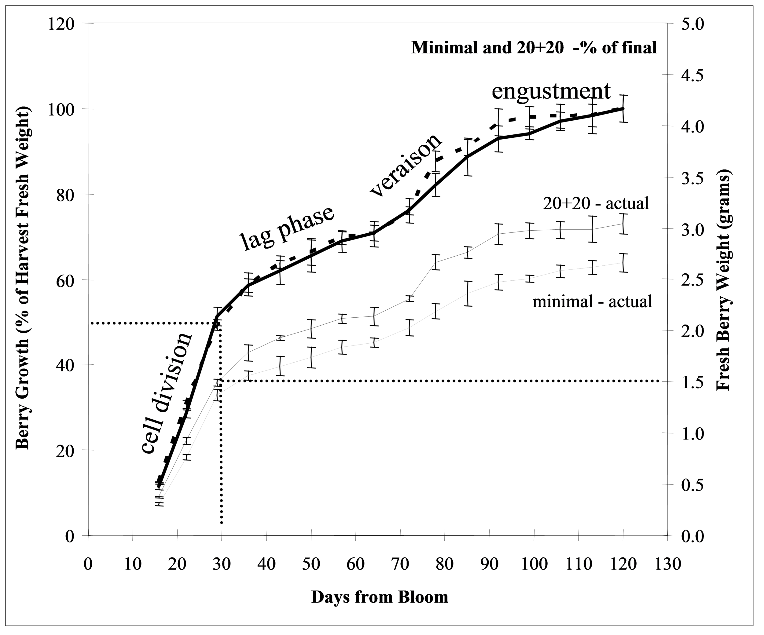
In 2014, we compared three different techniques for crop estimation at CLEREL and compared the estimates with the actual harvest weights from the processor scale house and a harvester-mounted grape yield monitor. First, we followed our developed method for sampling the vineyard by clean picking two panels (1% of an acre at our row and vine spacing), weighing the fruit from those two panels, and multiplying that weight by a berry weight factor to calculate a final harvest weight (Figure 1). At CLEREL, we did not address crop estimation until 50 days after bloom (not the typical 30 days after bloom) because of conflicts with other research activities; therefore, we were between 65-70% of final berry weight (not the typical 50% at 30 DAB).

Figure 1: Crop estimation sampling 30-50 days after bloom.  Approximately 1% of an acre is clean picked and weighed.  The current crop weight is multiplied by a berry weight factor and sample size factor to calculate a harvest estimate in tons/acre.  In 2014, crop estimation at CLEREL was done at 50 DAB (August 4, 2014), approximately 65-70% final berry weight, and we used a berry weight multiplication factor of 1.4-1.5 (100/70 = 1.43).

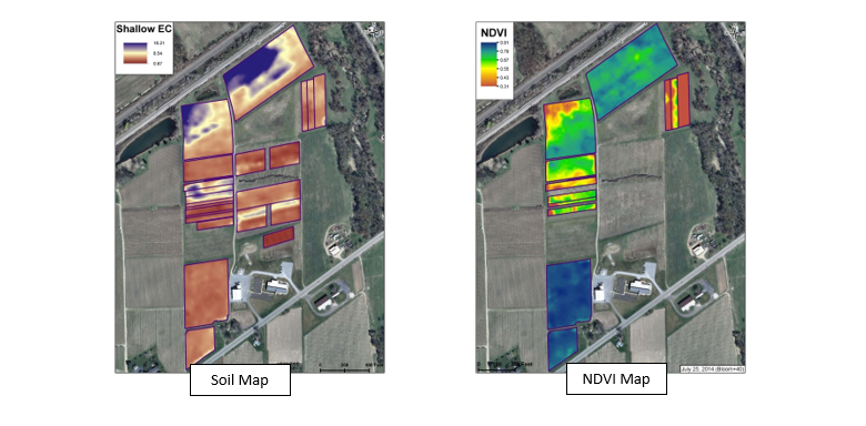
We collected 16 samples over 16 acres of grapes. Typically, this would be done randomly with the hope that the small sample size would accurately represent the whole vineyard. In 2014, canopy sensor measurements (NDVI) were collected at 20, 30, 40, and 50 days after bloom. The 20 DAB NDVI spatial map was used to designate three vine vigor classifications (low, medium, high). The 16 crop samples were stratified across the three classifications (Figure 2) and a mean crop estimate was generated for each classification.

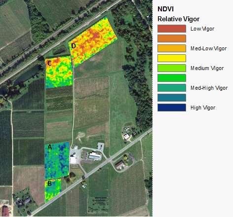
Figure 2: A map of CLEREL vineyards depicting the NDVI generated vigor classifications (colors) and sample locations (black dots).

The harvest crop estimate was calculated three ways: a single mean, three vigor classes, and continuous with NDVI (Figure 3). In the “single mean” method, the average from the 16 vineyard samples (8.57 tons/acre) was simply applied to the total acres (16.12 acres). In the “three vigor class” method, the mean from the samples in the low vigor zone was applied to the acres of the low vigor zone, the mean from the medium vigor samples was applied to the acres of the medium vigor zone, and the mean from the high vigor samples was applied to the acres of the high vigor zone. In the “continuous with NDVI” method, the

linear relationship between NDVI and predicted yield in the 16 samples was determined and the mathematical relationship was applied back to the spatial NDVI map to generate a spatial predicted harvest map and overall crop estimate. The harvest estimates were compared to the actual harvest weights collected from a harvester-mounted grape yield monitor calibrated against actual truck weights at the scale house.

The actual yield from CLEREL in 2014 was 133.8 tons (Figure 3). Using the single mean method and assuming crop estimation was done between 65-70% of final berry weight, the crop estimate was between 138-148 tons (3.3-10.6% high). The three vigor class method estimated between 133-143 tons (0.1-7.2% high) and the continuous method estimated 137-145 tons (2.5­9.8% high). Therefore, using the NDVI generated vigor zones and assuming 70% of final berry weight at 50 days after bloom (a berry weight factor of 1.4) gave the most accurate crop estimate.

Figure 3: Crop estimation and actual yield maps including the relationships used to calculate the estimates. The numbers represent the harvest tons estimated on 16.12 grape acres and the percent the estimate was off from the actual harvest weight.

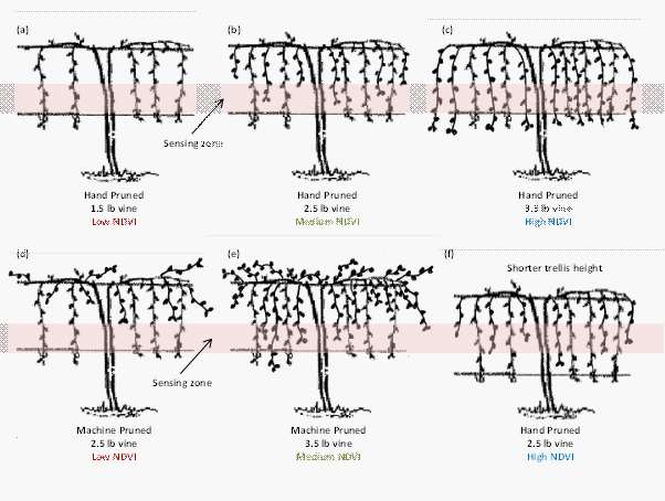
Similar to the curve-linear relationship between vine pruning weight and yield, vine yield increased with increasing NDVI values until the canopy was full and maximum light interception was reached. Higher NDVI values did not translate to higher yield. The “three vigor class” method, although coarse with only three means, approximated the actual curve-linear NDVI-Yield relationship more than the “continuous by NDVI” method, which assumed a strictly linear relationship. Therefore, the continuous method overestimated crop size at very high NDVI values.

Although we measured berry weight at crop estimation time and at harvest, it is interesting to note that we did not need berry weight measurements for any of these methods. We used the days after bloom and the standard berry curve in Figure 1 and made the assumption that the berries were 65-70% of final weight.

Economics of Sensor Driven Crop Estimation:

The commercialization of sensor technology requires a capital investment by the grower. Sensor packages used in this project are commercially available for $13,000. To cover 50% of the acreage in the region with this sensor package a total industry investment of $1.5 million would be required. The industry benefits of using this method of crop estimation, compared with grower results are likely to exceed $1 million in 2014. This is in a year when virtually 100% of the crop reached maturity. The economic impact of sensor driven crop estimation has much greater potential in higher risk years.

As our understanding of sensor technology advances, so to do potential uses. The use of sensor technology can decrease the cost of crop estimation by 50% or $2.50 per acre. While the cost of yield estimation is insignificant, a decrease in the labor associated with the practice increases the likelihood that growers will estimate their crop. A grower using NDVI to assist in crop estimation had a final crop size within 3% of their estimate.

For the Lake Erie Region, 2014 crop estimates were 80% of actual. Nationwide averages were 90% of actual. This creates serious financial and production risk to growers. Grower-owned processors incurred significant increases in containment costs that could have been avoided by simply understanding the size of the crop. In the Lake Erie Region, inaccurate crop estimation even resulted in the non-delivery of marketable tonnage. Further, there are also significant production risks associated with over-cropped vines that cannot be remedied unless the grower knows his crop size.

We have identified the $400,000 in costs to the industry. In all likelihood, because of proprietary processor information and return crops for 2014, the actual costs are significantly higher.

Concord Crop Adjustment: Theory, Research, and Practice

by Dr. Terry Bates

Viticulture Research Associate

Cornell University

Mechanical crop adjustment or “thinning” of Concord fruit has gained popularity in the past decade for various reasons, one being the integration of mechanical crop load management into mechanical pruning. In the past five years, we have conducted several research projects at the Cornell Vineyard Laboratory in Fredonia and in cooperating grower vineyards investigating the physiological and practical aspects of mechanical crop adjustment. Many area growers have tried thinning for themselves with varying degrees of success. The following article covers the theory behind crop adjustment, the information we have learned from our Concord research projects, and the practical method for in-the-field mechanical crop adjustment.

Theory

Sustainable productivity of both ripe fruit and mature wood depends on the appropriate ratio of exposed leaves to retained fruit, otherwise known as crop load. An undercropped vine (one with a lot of exposed leaf area to retained fruit) will have ripe fruit and excess vegetative growth. An overcropped vine (one with little exposed leaf area relative to retained fruit) will have delayed fruit and wood maturity leading to a decrease in vine size and future fruiting potential. There have been extensive arguments over the definition of vine balance. Most likely because the definition is different depending on the individual grower, processor, winery, grape variety, intended purpose for the fruit, or maturity characteristic being measured. For the purposes of this article, let’s assume that a “balanced” vine reaches a desired Concord fruit maturity of 16obrix by the middle of a typical harvest season while maintaining 2.5 to 3.0 pounds of cane pruning weight.

Since we can measure exposed leaf area, fruit weight, and juice soluble solids, we can determine the effect of crop load on fruit maturation in Concord (Figure 1). We conducted a series of crop and leaf thinning experiments to create a range of leaf area to fruit ratios in Concord vines pruned to 120 nodes. The vines were harvested during the middle of a normal harvest season and the crop load / obrix curve shows that desired fruit maturity was achieved when there was 15 square centimeters of exposed leaf area per gram of retained fruit. Undercropped vines (on the right side of the curve) did not have greater fruit maturity but tended to increase in pruning weight. Overcropped vines (on the left side of the curve) had lower fruit maturity and tended to have decreased pruning weight.

Figure 1. The effect of crop load (exposed leaf area to fruit ratio) on juice soluble solids in Concord.

For reference sake, in this particular vineyard block and growing season, 120 node unthinned vines yielded between 11 and 12 tons/acre, had a leaf area to fruit ratio of 10 and a fruit maturity of about 14.5-15.0obrix. Therefore the unthinned vines were slightly overcropped and either needed to be crop adjusted or needed an extended growing season to reach our desired fruit maturity of 16obrix. Thinning the vines down to 8-9 tons/acre increased the leaf area to fruit ratio to 15 and fruit maturity to 16-17obrix.

When I went back and looked at some of the old balanced pruning experiments by Dr. Nelson Shaulis and recalculated the leaf area to fruit ratio based on pruning weight data, I could illustrate why 20+20 pruning was so popular with Dr. Shaulis. Going back to figure 1, 10+10 balanced pruning had high leaf area to fruit ratios, were well undercropped, and tended to be over vigorous. In contrast, 30+30 pruning put the vines on the shoulder of the crop load / obrix curve. In good growing seasons, 30+30 vines were ideal with high yield, good fruit maturity, and adequate vegetative growth. However, in poor years, 30+30 pruning ran the risk of overcropping. A good option would be to crop adjust the 30+30 vines in poor years to increase the leaf area to fruit ratio and more appropriately match the crop load with the growing season. Dr. Shaulis used 20+20 pruning in many of his experiments and we still used 20+20 pruning in many of our current experiments that we do not intend to crop adjust. We do this because 20+20 pruning keeps us on the “safe” side of the crop load / obrix curve. In good years, the vines tend to be undercropped and will gain pruning weight and in poor years the vines will be balanced without going off the crop load cliff.

Research

The data from figure 1 indicated that balanced pruning and fixed node pruning with crop adjustment can both be used to manipulate crop load in Concord vineyards. Research over the past five years has attempted to address issues that put that theory into practice. Balanced pruning (especially to 20+20) is rare in commercial Concord vineyards because it can be labor intensive and it does not take advantage of the good growing seasons where a larger crop can be harvested without sacrificing wood maturity. Fixed node pruning is more common but can easily create an overcrop situation, especially where crop adjustment is not being considered. Machine assisted pruning with or without hand pruning follow-up also lends itself to fixed node pruning but again raises questions about appropriate node number and crop adjustment. Following our crop load theory and the goals of the Concord industry, efficient crop load management requires pruning for maximum crop for the best possible growing seasons and then crop adjusting down to match the vineyard potential with the particular growing season.

Surprisingly, pruning for maximum crop does not mean not pruning at all and it also does not mean leaving the same number of buds on all the vines in a particular vineyard. In a cooperative research project between NY, MI, and WA, Concord vines were pruned to a range of bud numbers and harvested at a pre-determined fruit maturity level. Interestingly, the plot in MI tended to have small vine size, the one in NY had medium vine size, and the one in WA had large vines (1.5, 2.5, and 3.5 pounds/vine, respectively). In each state, yield increased with increasing retained nodes to a point which I refer to as the yield plateau. The small vines reached a yield plateau at approximately 90 buds, medium vines at 120 buds, and large vines at 150 buds (Figure 2A).

Figure 2A and B. The effect of retained nodes on yield (A) and relative harvest date (B) of small (circles), medium (squares), and large (triangle) vines. Data are from the three-state Concord juice quality project on single wire trained vines. Harvest date in (B) is the number of days it took a treatment to reach 16obrix relative to balanced (20+20) pruned vines.

Pruning to a lower bud number decreased yield and increased the rate of fruit maturity – this simply follows our crop load discussion. Leaving more buds with hedge pruning or minimal pruning did not increase yield further because of yield compensating factors such as lower cluster and berry weights; however, excess buds further delayed fruit maturity presumably because of canopy inefficiency (Figure 2B). Therefore, when pruning for maximum crop it is important to prune to a bud number that gives maximum crop potential for a given vine size level but not to prune beyond that number.

At the Vineyard Laboratory, we have been researching the physiological effect of crop adjustment on 120 node pruned vines at 30 days after bloom. We prune to 120 nodes because we target 2.5-3.0 pound vines and our node number experiment (from figure 2) indicates that the yield plateau is reached at approximately 120 nodes. Each year we have recorded an inverse relationship between yield and obrix (figure 3A). Below 5 tons/acre, the vines are undercropped and there is no further increase in juice soluble solids with further fruit thinning (i.e. the vines are on the top of the crop load / brix curve in figure 1). From 5 to 11 tons/acre, juice soluble solids decrease as yield increases. Although growing season conditions will influence the slope of this curve from year to year, the general trend is that for every 2 to 3 ton/acre increase in yield there is a decrease in one degree brix. In practical terms, if you have a 10 ton/acre crop that is going to be 15obrix at harvest and you thin the crop down to 7-8 tons/acre, the crop will reach 16obrix at harvest.

In addition to and probably more important than the increase juice soluble solids with thinning is the response of wood maturity to thinning. There is a direct inverse relationship between yield and ripe nodes of periderm (figure 3B). Periderm counts are a mature bud measurement that is proportional to pruning weight. In our experiment, as the crop decreased from 11 tons/acre down to 0 tons/acre the number of mature buds increased (and the pruning weight increased).

Figure 3A and B. The effect of yield on juice soluble solids (A) and ripe nodes of periderm (B) on 120 node pruned vines at the Cornell Vineyard Laboratory in Fredonia. Each point is the mean of 10 vines, bars=standard error.

Other studies have shown that increasing vine size increases crop potential; therefore, thinning in year one not only influences fruit maturity in year one but also influences crop potential in year two by increasing vine pruning weight.

In the specific example in figure 3A and B, our goal was to harvest between 16 and 17obrix and maintain the vines between 450 and 500 ripe nodes of periderm (roughly 2.5 pounds of pruning weight) – our own specific vineyard balance definition. At 11 tons/acre, the fruit was harvested at 15obrix and periderm counts were around 400. Fruit thinning down to 7-8 tons/acre increased the fruit to 16.5obrix and 475 ripe nodes of periderm, thus achieving our goal for vineyard balance. Thinning below 7 tons/acre turned out to be excessive thinning in that particular vineyard and growing season.

I am always drilling home the importance of vine size on Concord productivity. It is no surprise that vine size also influences the thinning response in Concord. In 2002, we repeated the 120 node thinning experiment on small, medium, and large vines.

The yield/brix regression lines in figure 4A show that small vines were more responsive to thinning than medium or large vines. Calculated exposed leaf area to fruit ratios (Figure 4B) also show that the crop load / obrix curve is the same for all vine size categories; however, at a given yield level the vines will be at a different points on the crop load / obrix curve. Or, the vines will reach similar leaf area to fruit ratios at different crop levels.

What about timing? Typically, commercial Concord vineyards are mechanically crop adjust at 30 days after bloom; however, other thinning times have been tested or considered. Dr. Shaulis used manual flower cluster thinning in the West Tier back in the 1960’s. Unfortunately, thinning prior to fruit set can increase the percent of florets that set fruit leading to some degree of yield compensation. In theory, the earliest that the crop can be adjusted after fruit set, the more efficient the vine response will be because the vines have invested few resources into the crop. In practice, the berries have little mass right after fruit set and it is difficult to accurately fruit thin with a machine when the berries are that small.

Figure 4 A and B. The effect of crop level (yield-A) and crop load (exposed leaf area to fruit ratio-B) on juice soluble solids of small, medium, and large Concord vines pruned to 120 nodes.

Dr. Pool investigated Concord berry growth in relationship to both calendar days after bloom and growing degree days. His research showed that Concord berries reached 50% of final fresh berry weight approximately 30 days after bloom and more specifically at 1200 growing degree days. The “50% final berry weight/30 day after bloom” timing has been adopted by several growers as a convenient time to both estimate the crop and mechanically crop adjust.

Growers have also asked about thinning later in the season (50 days after bloom) when berry growth slows down during the lag growth phase (Figure 5). At 30 days after bloom, fresh berry weight is rapidly changing and a few days in either direction can cause large errors crop estimation. At 50 days after bloom, the rate of fresh berry weight change is smaller when compared to the rate of change at 30 days after bloom, potentially providing added flexibility and accuracy to crop estimation. However, there should also be a resource cost associated with leaving an excessively large crop on the vine for an extended time period.

Figure 5. Typical Concord berry growth curve showing both actual and % of final berry weight for balanced (20+20) and minimal pruned vines.

In 2002, we conducted another thinning experiment in 120 node vines at the Fredonia Lab where we manually crop adjusted at 20, 30, 50 days after bloom, immediate pre-veraison, and 2 weeks post-veraison.

Figure 6A and B. Juice soluble solids accumulation from veraison to harvest on vines with different crop levels prior to veraison and on vines thinned 2 weeks post-veraison (A). The effect of yield on final harvest juice soluble solids of vines thinned at various times pre-veraison and 2 weeks post-veraison.

In terms of juice soluble solids accumulation, all of the pre-veraison thinning times led to a similar increase in obrix at a given crop level. Fruit from all treatments in the experiment started at approximately 7obrix at veraison (figure 6) The rate of soluble solids accumulation in vines with 50% crop was greater after veraison than on vines with 75% or 100% crop. Vines thinned two weeks after veraison had a slow initial rate of soluble solids accumulation (similar to vines with 100% crop). After thinning 2 weeks post-veraison, the rate of soluble solids accumulation increased until harvest (similar to vines with 50% or 75% crop). The post-veraison thinned vines were unable to catch up to the earlier thinned vines by the selected harvest date (figure 6B). In theory, all data curves in figure 6A would eventually merge into one line if the growing season were long enough. The practical problem is that an extended harvest season is a rare luxury in the Lake Erie grape belt.

As discussed earlier, crop adjustment is important for both fruit maturation and wood development. Concord growth analysis research that we have done shows that perennial grapevine tissues accumulate starch approximately one month after bloom until the end of the growing season. It could be argued that delaying crop adjustment later than 30 days after bloom would infringe upon early wood development through the partitioning of resources, such as carbon and nitrogen, into a the crop.

Figure 6A and B. Juice soluble solids accumulation from veraison to harvest on vines with different crop levels prior to veraison and on vines thinned 2 weeks post-veraison (A). The effect of yield on final harvest juice soluble solids of vines thinned at various times pre-veraison and 2 weeks post-veraison.

Figure 7. The effect of thinning time on final vine pruning weight of small, medium, and large vines.

Pruning weight data from different sized vines thinned to 75% crop level at five different timings during the growing season brings our whole discussion of crop adjustment together. On already large vines, thinning time did not have an effect on final vine size (figure 7). The large vines had a relatively high leaf area to fruit ratio at a given crop level when compared to medium or small vines (as seen in figure 4); therefore, the large vines in our experiment could mature both the fruit and wood well within the limit of the growing season.

In contrast, small vines with relatively low leaf area to fruit ratios (higher crop load) at a given crop level had lower juice soluble solids accumulation rates (figure 4) and were affected by thinning time (figure 7). In general, delaying crop adjustment decreased vine pruning weight and this response was measured as early as 30 days after bloom.

Conclusions:

1) Vine response to crop load is the same whether crop load is manipulated by pruning, thinning, or a combination of the two.

2) In an average growing season with average vine size, Concord vines require 15 square centimeters of exposed leaf area per gram of fruit fresh weight for balanced production. Vines with a lower leaf area to fruit ratio need crop adjustment or an extended growing season to maintain a balance between vegetative and reproductive growth.

3) In overcropped vines, thinning increases both juice soluble solids and vine pruning weight. The response is more pronounced on small vines than on large vines because small vines have a higher crop load than large vines at a given crop level. On small vines, thinning approximately 2 tons/acre leads to an increase in one degree brix. On large vines, thinning approximately 3 tons/acre leads to an increase in one degree brix. On undercropped vines (below 5 tons/acre), there is no effect of thinning on juice soluble solids.

4) In terms of thinning time, thinning can be done any time before veraison to increase the juice soluble solids accumulation rate in the remaining fruit. In terms of wood maturation, thinning time impacts small vines more so than large vines. In commercial vineyards with lower than optimum vine size and/or with a variety of biotic and abiotic stresses, crop adjustment should be done as early as practically possible so that the crop load change can have a larger increase on wood development. On large healthy vines, thinning time did not impact the resultant vine size (although I question if this statement remains true if the same vines are pushed and thinned late for several years in a row).

Practice

Everyone is always asking me how our research translates to commercial vineyards. In-the-field mechanical thinning research has been going on in the Lake Erie region since the early 1990’s. I have been involved with several growers, especially Bob and Dawn Betts, Joel Rammelt, and Dave Vercant, for the past five years evaluating on-farm mechanical thinning. Our research shows that mechanical crop adjustment, if done correctly, gives the same results as thinning at the Fredonia Lab (figure 8). We have used different harvesters and thinning heads with straight rods and bow rods and at different thinning speeds.

Figure 8. The effect of yield on juice soluble solids of hand thinned 120 node vines (same as figure 3A) compared with two thinning machines at two thinning rates. Canopy damage only impacted fruit maturity when we tried to thin approximately 8 tons/acre.

Many growers have reported that they have beat up their vines with mechanical thinning and it is certainly possible to cause significant canopy damage when thinning. However, we have found that with some common sense and a little machine operation experience that this damage can be avoided. Some useful tips are. . .

1) Bring your common sense. If it looks like you are taking off more leaves than fruit or causing significant canopy damage, you probably are. Adjust your thinning machine.

2) Avoid having to thin off more than 3-4 tons. If you have a vineyard that can yield 8 tons/acre in an average year, use dormant pruning to target 10 tons/acre in the prospect of a good growing season. Then thin off a few tons if the year is less than perfect. Avoid hanging 15 tons/acre and then having to thin off 7 tons/acre – it always leads to poor results.

3) Shake – don’t slap! Machines that grip and shake the canopy tend to cause less canopy damage than those that slap the foliage and break shoots. Floating picking heads and bow rods are nice features to some new machines but they are not mandatory. We have had excellent results with the correct set up of old machines and straight harvester rods.

4) Some like it Hot! We have found much less shoot breakage on Concord when thinning is done during a warm afternoon. First thing in the morning, the shoots are pumped up with water and tend to break during thinning. At 30 days after bloom in mid-July, the warm afternoon temperatures cause the shoots to relax and become more flexible later in the day resulting in less shoot breakage.

5) Talk to your fellow growers that have thinned successfully. They are a wealth of practical information.

How to Mechanically Crop Adjust: The Easy Method

The following method considers mechanically crop adjusting at 30 days after bloom with “playing all the averages.” The easy method takes less thought but can also be less accurate because it takes into account several assumptions.

To successfully crop adjust; a grower needs to know what the balanced cropping potential is for a particular vineyard block in an average growing season. For example, a grower knows that Block A is in a poor spot and can only handle 5 tons/acre and that Block B is in a good spot and can run 8 tons/acre in an average growing season without loosing significant pruning weight. Next, all the grower needs to do is measure what crop is hanging in the vineyard and adjust the harvester to take off the excess crop to reach the target crop level.

To crop estimate using the easy method, 1% of an acre is clean picked and weighed at 30 days after bloom. At 9 foot row and 8 foot vine spacing, there are 605 vines in one acre. A row of 605 vines at 8 foot spacing would be 4840 feet long. 1/100th or 1% of that row would be 48.4 feet. An easy way to pick 1/100th of an acre is to measure and cut a piece of rope 48 feet long, lay it down on the vineyard floor, and clean pick the vines in that rope length with a harvester. The picked green berries are then sent across the harvester shoot to a barrel on a scale (many growers use a milk scale on a trailer). Weight the picked fruit. In the easy method, simply read the weight of the fruit picked off of 1/100th of an acre (in pounds) and move the decimal point over one place to the left to get the harvest estimate in tons/acre.

For example, in Block X, Bob lays out his 48 foot crop estimation rope (roughly two post lengths) and clean picks it. Dawn, on a trailer in an adjacent row, places a barrel on a milk scale, tares (or zero’s) the scale, collects the berries from the harvester shoot into the barrel, and weighs the green fruit. The scale reads 100 pounds. Dawn moves the decimal point one place to the left and estimates that the block will have 10 tons/acre at harvest. Bob and Dawn repeat the procedure in a Block Y and the scale reads 50 pounds. They estimate that they will harvest 5 tons/acre from Block Y.

Bob and Dawn decide that Block Y with the 5 tons/acre estimate does not need thinning and they leave it alone. Block X, on the other hand, has a 10 tons/acre estimate and they want to thin it down to 8 tons/acre by taking off a harvest equivalent of 2 tons/acre. Working backwards and moving the decimal point one place to the right, Bob and Dawn must set up their harvester to remove 20 pounds of fruit in the same 1/100th of an acre (48 feet). After a couple trial runs at different beater speeds, they are comfortable that they are taking an average of 20 pounds of fruit off of a 48 foot section. Bob then runs over the rest of the block with the determined machine set-up.

How to Mechanically Crop Adjust: The Advanced Method

The easy crop adjustment method assumes that thinning is done at 30 days after bloom, that the berries are at 50% of final berry weight at 30 days after bloom, and that there is an average growing season. The actual physical activity in the vineyard between the easy and advanced methods is the same – pick 1/100th of an acre and make some decisions about thinning. However, the advanced method takes into account actual berry weight and growing season conditions to make more educated decisions in the vineyard and to decrease error in the thinning process.

The way I like to calculate % final berry weight in crop estimation is to weigh a berry sample at the time I am thinning and make a prediction on what the final berry weight is going to be. I do this for three reasons: 1) the berry weight at 30 days after bloom and at the end of the season is different every year (is there such a thing as an average year?); 2) the berry weight is changing very fast in the 30 day after bloom / 1200 GDD period (see figure 5); 3) I am not always crop adjusting at exactly 50% of final berry weight in any one vineyard or any one area in the Lake Erie Belt.

1. Clean pick 1/100th of an acre (as in the easy method) and weight it.

Example: 142 pounds of green fruit is picked from 48 feet.

2. Measure average fresh berry weight at thinning time. Typically I weigh a couple different 100 berry samples to get a reliable average berry weight at thinning time.

Example: Average berry weight measured at 1.8g.

3. Predict what you think the final berry weight will be at the end of the season. This can be tricky but I feel that it is more accurate than automatically assuming that the berries are at 50% final berry weight.

Rules of thumb: Final berry weight changes with crop level, pruning method, and growing season. Balanced pruned vines with relatively light crops average 3.0g berries at harvest. 120 node vines average 2.75 g berries and Minimal pruned vines average 2.5 g berries at harvest (see figure 5). Excellent growing conditions with adequate water during the cell division phase of berry growth lead to larger than average berries. Lack of water post-veraison can lower final predicted berry weight. Predicting final berry weight is a guess at best and will always add error to the crop estimation (however, cluster and berry counts are old crop estimation errors that are now removed from the procedure).

4. Calculate % final berry weight.

Example: If average berry weight is 1.8g when I am going to thin and I predict that the final berry weight is going to be 2.75g then I calculate that I am at 65.4% of final berry weight (1.8/2.75 = 0.654 or 65.4%).

5. Calculate the multiplication factor for crop estimation.

Example: If I am at 65.4% of final berry weight then I should multiply my 1/100th of an acre sample by 1.53 (100/65.4 = 1.53) to get what the sample will weigh at harvest.

6. Calculate the per acre crop estimate.

Example: 142 pounds of green fruit multiplied by 1.53 = 217.3 pounds of fruit in 1/100th of an acre at harvest. This is equal to 21730 pounds of fruit per acre at harvest (217.3 x 100 = 21730) or 10.87 tons/acre (21730 / 2000 pounds per ton).

7. Determine the desired crop level for the vineyard block. As in the easy method, if the grower knows a vineyard block is balanced at 8 tons/acre then that yield can be targeted each year. However, at the vineyard lab we look at the growing degree days at thinning time and make a judgment on how much crop to leave based on how many days we are ahead or behind average. The rule of thumb: For every three days ahead of average we are at thinning time we can ripen one ton/acre more than average. This “3 day per ton” rule comes from a Concord pruning experiment where vines with a range of crop levels were harvested based on juice soluble solids and not on a single date.

Example: If a vineyard can ripen 8 tons/acre on an average year and we are a week ahead of average at 30 days after bloom then we would predict that the same block can potentially ripen 10 tons/acre. In contrast, if we are a week behind average at 30 days after bloom then we would predict that the same vineyard block may be better balanced at 6 tons/acre. The only downfall to this rule of thumb is if the weather drastically changes between thinning time and harvest. However, I am more comfortable making weather related crop load decisions one month after bloom than I am in the middle of January when crop load is being decided with pruning alone.

8. Work backwards to determine the machine set up for thinning.

Example:To shake off 2 tons/acre harvest equivalent when the berries at 65.4% of final berry weight.(2 tons/acre x 2000 pounds/ton = 4000 pounds/acre = 40 pounds in 1/100th of an acre at harvest.40 pounds / 1.53 berry weight multiplication factor = 26.14 pounds of green fruit to remove from 1/100th of an acre at thinning time).

9. Set-up machine to take off desired amount of fruit.Unfortunately, with all the different machines and harvester configurations out there, this is still a trial and error process. The set-up with a Chisholm-Ryder with straight rods is different than a Morris-Oldridge thinning head or a Korvan with bow rods.

The Basics of GIS and NDVI and Their Use in the Vineyard

by Rhiann Jakubowski

Anyone who has been in contact with the Lake Erie Regional Grape Program (LERGP) within the last few years has probably heard the terms “NDVI” and “GIS” used quite frequently. With all of the discussions about vineyard mechanization and precision viticulture, what are NDVI and GIS, and what are some of the applications that are pertinent to those in the grape industry?

GIS:

What is it?

A Geographic Information System (GIS) is a system that allows for spatial, or geographic, data to be interpreted in a digital format. In this way, data can be more easily stored, shared, manipulated, analyzed, and understood. For our purposes, you will hear me use the phrase “GIS” to describe a computer program, ArcGIS (developed by ESRI). ArcGIS is a platform that allows the user to create, load, and overlay datasets in a variety of ways. When you hear “GIS”, think “maps”!

How is it used at LERGP?

We began the GIS Mapping Project back in 2011 at LERGP as a way to gain a better understanding of the distribution of vineyards and grape varieties throughout the Lake Erie grape belt. Since then, the vineyard polygons GIS layer has been an invaluable resource for research and extension projects at CLEREL.

One of the most notable projects is the collaboration between the Lake Erie Regional Grape Program and National Grape Cooperative to provide all members (of either organization) with accurate acreage maps of their vineyards. These maps are considered the foundation of precision viticulture as more layers of data (NDVI, soil, elevation, etc.) can be overlaid in order to interpret underlying relationships within specific vineyard blocks.

GIS has also been used to map the relationships between frost events and bud damage in 2012, as we split the region into distinct growing zones based on field-collected data. We will be exploring the effects of the severe cold events in February of 2015 on bud damage in a similar manner utilizing our GIS resources.

NDVI:

What is it?

Normalized Difference Vegetative Index (NDVI) is a formula that is used to quantify the density of plant growth in a particular area. No green leaves results in an NDVI value of zero, while healthy, dense leaves result in an NDVI value near +1. Chlorophyll, the green pigment in plant leaves, strongly absorbs visible light during photosynthesis. However, near-infrared light is strongly reflected by the plant’s cell structure. As a result, the more photosynthesizing leaves that a plant has, the more the Red and near-infrared (NIR) wavelengths of light are affected, thus changing the NDVI value.

To keep it simple, when you hear “NDVI” think of “green leaf area”!

How is it used at LERGP?

For the past few years, LERGP has been collecting NDVI readings from research and grower vineyards during various times throughout the growing season to discover if there is a relationship between vine vigor, yield, and crop load. Using the results from the NDVI canopy sensing combined with the data from soil sensing, our viticulturalist, Luke Haggerty, can help growers to make educated management plans to reduce variability within vineyard blocks and increase vine productivity. Remember, the NDVI sensor will not tell you why vigor is low; it will only show you that canopy size is different within your block.

The NDVI sensors are mounted on a tractor, gator, or other piece of machinery and driven through a vineyard on an every-other-row or every-third-row pattern, with the sensors aimed at the growing region of the vines. The data collected is then processed at the lab using GIS and other computer programs to create a map that the grower can use to visualize variability within the vineyard. This information has proven especially useful during crop estimation sampling or other directed sampling.

Canopy Sensing Facts Sheet; Adapting Canopy Sensing Systems

by James Taylor,

The team at CLEREL is researching and developing methods to incorporate information from high-resolution canopy sensors into Concord (and Niagara) production systems. Two sensing systems are being trialed; the N-Tech GreenSeeker and Holland Scientific CropCircle. These canopy sensors operate by measuring the reflectance of visible (Blue, Green and/or Red) and Near Infra-Red (NIR) light from the leaves. The amount of reflectance is dependent on i) the number of leaves and ii) the health (color and cell structure) of these leaves.

By measuring the canopy response and looking at the variation within a field or vineyard, it is possible to identify areas of low, medium and high vigor vines. Understanding this variation within a field, will provide information that allows growers to quantify (properly measure) under producing areas and the cost of potential lost crop production.

What does the NDVI (Normalized Difference Vegetation Index) mean?

The most common way that the information from canopy sensors is displayed is as a Normalized Difference Vegetation Index (NDVI). The NDVI value is a ratio between the reflectance of Red and NIR from the canopy. Healthy green plants absorb Red light for photosynthesis (i.e. they have a low Red light reflectance), but strongly reflect NIR light. Good leaf cell structure (again indicating healthy plants) leads to higher NIR light reflectance. Therefore vigorous plants should have a low Red and high NIR light reflectance while weak plants will have a relatively higher Red and lower NIR light reflectance. The ratio between Red and NIR therefore forms a good basis for identifying low and high vigor plants based on their canopy reflectance.

Sensor operation

In a practical sense, canopy sensors are operated by imaging (pointing at) the part of the vine where differences in vine growth are expected. Early in the season the sensor can be directed at growth around the top wire cordon (Figure 1a). At this stage of growth the sensor will differentiate between weak and strong early season growth. As the season develops, all vines develop a thick canopy around the top wire. This leads to a saturation of the sensor signal. When the canopy is complete along the top wire there is little or no difference in the sensor response between low and high vigor vines.

At this stage the sensor can be moved from imaging the top wire to imaging the side-curtain of the vines. Typically the sensor should be mounted about 18 inches above the ground (around the bottom wire if present) (Figure 1b). The rationale here is that vigorous vines will have a well-developed side-curtain with long canes that will present a large amount of leaf to the sensor low down on the side-curtain. Weaker vines, with fewer and/or shorter canes will have less leaf material in the same area. Examples of these differences are shown with photos from a vineyard in Figure 2. The difference in side-curtain development allows the sensors to map differences in vine vigor.

Figure 1: Examples of a canopy sensor being used (A) early in the season to sense early season development and (right) late in the season to sense differences in the canopy side-curtain development.

Figure 2: Photos of the difference in side canopy development in (A ) low vigor and (B) high vigorvines within a Niagara block at CLEREL.

Interpreting NDVI maps

NDVI is a normalized or relative response. The sensor output will be very dependent on how the canopy (vine) is presented to the sensor. As stated above, if the top wire is imaged late in the season, then the sensor will always see a full canopy and will interpret all vines to be of high vigor. The schematic presented below (Figure 3) shows how the sensor response may differ with different canopy architectures. On the top line of Figure 3 it is easy to see how imaging the side canopy (the red zone) shows an increase in sensor response (from low to high NDVI) as vine size increases from 1.5 to 3.5 lbs/vine. The example here is in a hand-pruned vineyard on a constant 6 foot high trellis. The second line in Figure 3 shows some alternate canopy architectures. Machine pruning tends to generate a greater canopy density along the top wire than hand-pruning. Consequently, the side-curtain may be less developed than in hand pruned vineyards for a similar sized vine. Both vines (b) and (d) are 2.5 lbs. vines but the NDVI response from imaging low down on the canopy side-curtain will be relatively lower in the machine pruned vineyard. This is only due to the difference in canopy architecture between hand and machine pruning, not a difference in vine size or productivity. The same can be seen for vines (c) and (e) that are both 3.5 lbs. vines, but again differ in pruning management and NDVI response. A change in the trellis system will also affect the sensor response. Vines (b) and (f) are both 2.5 lbs. vines; however the trellis height for vine (f) is shorter so that the relative position of the canopy sensor is closer to the top wire. As a result, vine (f) presents more foliage and an apparently higher NDVI for the same size vine with the same pruning management. Note also the difference in NDVI response between the taller trellis machine pruned vine (d) and the shorter trellis hand pruned vine (f). Both vines (d) and (f) have the same pruning weight.

Keypoint: Management will affect the relative sensor response. The patterns in the NDVI maps should only be interpreted within a single block or between blocks that have the same management!!

Figure 3: A schematic diagram to illustrate how the response of a canopy sensor that is sensing
along the bottom trellis wire may be affected by differences in pruning strategies and trellis set-up.

Comparing the NDVI response between blocks with a different variety, different pruning regime or different management is very difficult and can lead to misinterpretation. It should not be done. The main interest is to look for patterns within a block or within uniform management areas that indicate where vine vigor (size) is relatively small or large. If desired, the canopy sensor data can then be calibrated to a pruning weight by taking pruning weight measurements within the block. Otherwise, the patterns in the NDVI can be used to target sampling (soil, petiole etc.) to identify production limiting factors in the low vigor areas and (hopefully) remedy these factors. The effect of management can be illustrated with real data on the NDVI response from the juice grape blocks located at CLEREL, Portland (Figure 4). There are four large juice grape blocks at CLEREL – 3 Concord blocks (Blocks A, B and D) and 1 Niagara block (Block C). The response between the Concord blocks A (very vigorous) and D (low vigor) is very different. Without any information on these production systems it may be assumed that Block A is much more productive than Block D. However the difference in NDVI is in large part due to the fact that Block D is machine-pruned whilst Block A has been very carefully hand-pruned for the past 4 years. Consequently the presentation of the canopy to the canopy sensor differs in the two blocks and the difference in the NDVI signal is, therefore, not necessarily reflected in the production (yield) response (see Figure 3). The intensive hand-pruning in Block A has been done to ensure that the canopy side-curtain is fully developed in an ‘ideal’ hand-pruned system. This level of attention is obviously not feasible in (large) commercial production systems, which are increasingly adopting machine-pruning approaches.

Figure 4: The NDVI response for the juice grape blocks at CLEREL Portland. Blocks A, B and D are Concord, Block C is Niagara.

Keypoint: The canopy sensor data tells you where to look to identify problems in the vineyard. It does not tell you why vine vigor is low. Some agronomy and management expertise is needed to interpret the patterns and develop a management strategy for the observed variation in vine vigor.

During the 2012 growing season the team at CLEREL imaged ~ 750 acres of single wire top-wire trained Concord grapes in the Lake Erie region. This included vineyards from the east (Sheridan) to the west (Harborcreek) of the grape belt and vineyards, ranging in elevation from the lakeshore to the escarpment and included hand and machine-pruned vines. Over the coming months, work will continue to measure pruning weights within these vineyards to establish calibration curves between the NDVI response and vine size. This will allow the canopy sensor response to be converted to a site-specific pruning weight (vine size) estimation across a range of different management environments.